Copy to clipboard
Reader Question: Larger companies have statisticians on staff to determine the minimum number of samples for given validation and verification (V&V) activities, but for folks who don’t use Minitab and don’t have an extensive stats background, are there guidelines to know the right amount of parts to test?
Years ago, 30 parts was the golden number for V&V activities, but that seems to have become unacceptable in the past few years. Can we base sample sizing on average lot size, or are there easy process capability equations we can use to cut the waste we produce to validate a process and verify parts?
In the end, we want to have confidence in our V&V activities, but taking the conservative route on sample sizes for these activities can be quite burdensome. Our conservative approach is to test a large sample size based on a T-test or batches of 60 if we’re verifying an attribute.
For years, device companies used the Central Limit Theorem (CLT) and its rule of thumb of 30 parts tested. Increasing tolerances and regulatory oversight are two reasons that CLT is no longer relative. For example, FDA now seeks a more analytical approach—justification—for choosing sample size.
However, calculating an appropriate minimum sample size is one of the most difficult things to do and is an ongoing challenge for many of us. To complicate things further, a large number of journal articles are devoted to this subject, and their advice is often case-specific or discusses a new and unique way to determine a sample size, leaving us more confused than ever. I am not a statistician, and after reading a dozen or more articles, I’ve come to the conclusion that “everything depends on everything” when it comes to statistics. There are no simple answers.
That said, a couple of basic approaches should work in most situations. If your lot sizes are relatively large, as in on the order of 1,000 units per lot, and you have some history with the product so that you can define some acceptance parameters, then you can use either the acceptance sampling approach or the six sigma acceptable error approach to determine a sample size using statistics. I’ve discussed both approaches below.
Acceptance Sampling Approach
One way to determine sample size is to look at lot quality assurance. Acceptance sampling is based upon the probability that finding a defective part will occur less than or equal to a predetermined critical value for defects. For this method, the sample size, n, and critical value (number of defects found), d, depend upon parameters you establish for:
N—lot size
Pυ—upper threshold beyond which an intervention is deemed necessary (probability)
PL—lower threshold beyond which an intervention is deemed unnecessary (probability)
α—Type I error of concluding lot is acceptable when it is not, where α is set to as low a value as is deemed reasonable by the experimenter, often called a false negative
β—Type II error of concluding lot is unacceptable when it is fine, often called a false positive
Thus, (1-α) is called the sensitivity of the test to detect defective product and (1-β) is called the selectivity of the test in your decision making parameters. Obviously, a false negative is more dangerous than a false positive, but the more confidence you require in your inspection or test, the higher the rate of false positives you will have and the more samples you will need to inspect.require in your inspection or test, the higher the rate of false positives you will have and the more samples you will need to inspect.
Much of the literature for this approach discusses the operating curve (OC), which is a tool for determining sampling size based on the parameters defined above. You can find these curves from many sources. For each combination of n and d, the resulting OC curve (sometimes called a candidate sampling plan), provides the following information:
- The horizontal access is the proportion of product that is defective and ranges from 0 to 1.
- The vertical access is the probability of making a Type I false negative error for that candidate sampling plan. These values also range from 0 to 1.
- The slope of the OC curve tells us how the probability of making a Type I error changes as we vary our value of Pυ. The steeper the slope, the higher the power; however, the OC curve must also have a high sensitivity to α and must include data points up to the value of (1-α) in order to detect a Type I error.
A final consideration is statistical power. The power of a test is given by (1-β)*100%, with 80% being a standard value; however, a trade-off exists between a feasible sample size and adequate statistical power. Statistical power (think of in terms of sensitivity) is the probability that your statistical test will indicate a significant difference when there truly is one. This is frequently performed with α = 0.05.
As an example, let’s assume our goal is to calculate appropriate values of n and d that limit the chance of making a Type I error for a specified choice of α. You can find countless tables that will provide the resulting values of n and d based upon desired input values of α, β, Pυ, and PL. If you only consider α = 0.05 with d = 0 defects, for a lot size of 1,000, you will need 49 samples, according to one table I found. If you need to consider Type II, false positive errors as well, then you must include β and PL. For example, from one article I looked at, for α = 0.05, β = 0.20, Pυ = 0.05, and PL = 0.005, you would need n = 87 samples to get d = 0 defects for a lot size that is “large” (which I assumed to mean at least 1,000).
Six Sigma Error Approach
For this approach, in order to determine your sample size, you first have to measure your process capability. For example, this can be the diameter of a bolt or the tensile strength to failure or any other variable of interest. Whatever it is, you can determine the sample mean, x. This is going to be different than the true (or population) mean, µ, which could only be calculated by measuring every component. The maximum difference between the sample mean and the population mean is called the error, E, and is defined as:

In this formula, Z is the critical value, σ is the population standard deviation you’ve estimated over time and n is the sample size you’re trying to determine.
First, you need to define a critical value, Z. This is based on α, which is the area under the two tails of a normally distributed bell curve, with each tail being α/2. For most studies, α = 0.05, so α/2 = 0.025. Alternatively, you can think of this as a confidence interval of 95%, which is (1-α)*100%. Using the value of 0.025, you can look up Z in a table.
As an example, let’s say you want to determine the sample size if the standard deviation over time has been σ = 0.02 inches from the desired perfect length, but you’re willing to accept an error of 0.005 inches from that number for any given sample mean. Since we’re assuming normal distribution and we know probabilities vary from 0 to 1, the center of your bell curve is 0.5. Thus, you take 0.5 – 0.025 = 0.475 and look up Z = 1.96. Rearranging your equation to solve for n:
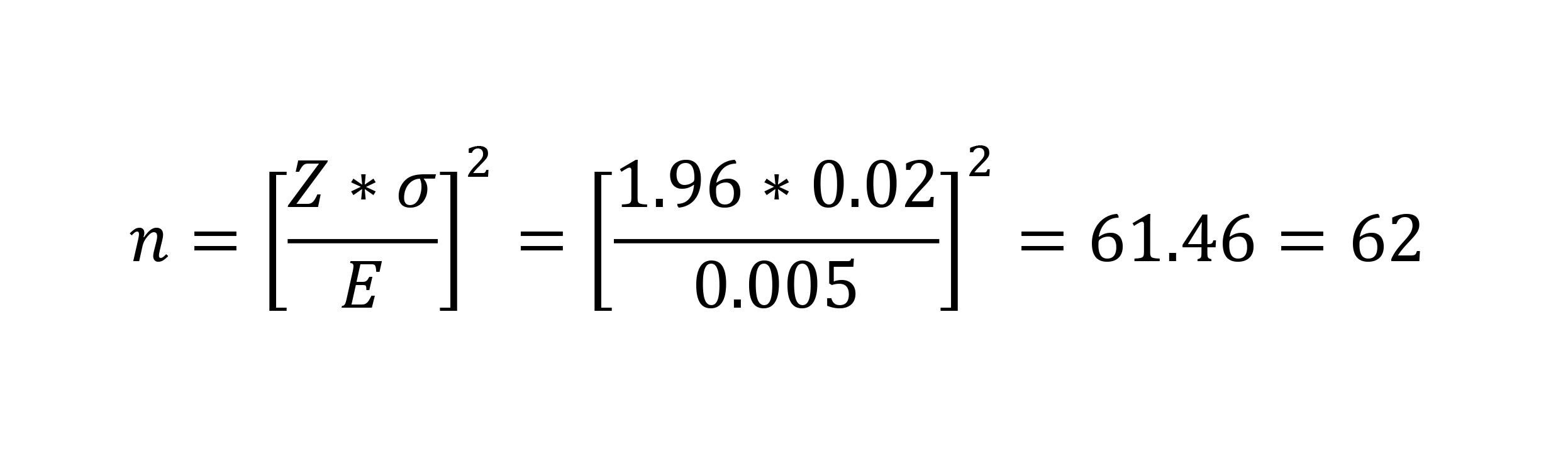
Thus, for this one measurement, your sample size should be 62. The formula is very sensitive to E, and this is something that you have to decide based on your experience. Note that it’s not necessary to do this calculation for every variable. In fact, you should choose your worst case, most important variables and set the sample size based on them, as all of the other variables will require fewer samples.
These are two possible approaches, although many more exist. Unfortunately, choosing a sample size is a judgment call based on many parameters and decisions you make. For either of the approaches above, I recommend that you vary the parameters to find an optimized solution, seeing how each of your input requirements effect your output quality and confidence levels.
Dr. Deborah Munro is the President of Munro Medical, a biomedical research and consulting firm in Portland, Oregon. She has worked in the orthopaedic medical device field for almost 20 years and holds numerous patents, mostly in the area of spinal fusion. She taught mechanical and biomedical engineering at the University of Portland for eight years, where she also founded a Master’s in Biomedical Engineering program. Her current interests include developing new medical device solutions for companies and assisting them in their regulatory compliance efforts. She can be reached by email.